Slicing Through Your Data: A Step-by-Step Guide to Creating and Using Slicers in Excel for Interactive Data Analysis

Slicing Through Your Data: A Step-by-Step Guide to Creating and Using Slicers in Excel for Interactive Data Analysis


Creating slicers in Excel allows you to filter and interactively analyze data in a visual and user-friendly manner. Here are the steps to create slicers in Excel:


Step 1: Prepare Your Data

  • Ensure that your data is well-organized in a table or range, with column headers and consistent data formats.


Step 2: Select Your Data

  • Highlight the data range or table that you want to work with.


Step 3: Insert a PivotTable

  • Go to the “Insert” tab in the Excel ribbon.
  • Click on the “PivotTable” button. A dialog box will appear.


Step 4: Choose Your PivotTable Source

  • Ensure that the “Select a table or range” option is selected in the dialog box.
  • Verify that the correct data range or table is automatically detected.
  • If necessary, manually adjust the range or select the entire table.


Step 5: Design Your PivotTable

  • In the PivotTable Field List pane, drag and drop the desired fields into the “Rows” or “Columns” areas.
  • If you want to summarize data, drag the desired field(s) into the “Values” area.


Step 6: Insert Slicers

With the PivotTable selected, go to the “PivotTable Analyze” tab in the Excel ribbon.
Click on the “Insert Slicer” button. A dialog box will appear.


Step 7: Select Fields for Slicers

  • In the dialog box, check the box(es) next to the field(s) you want to create slicers for.
  • Click on the “OK” button. Slicers for the selected field(s) will be added to your worksheet.


Step 8: Customize Slicers

  • With the slicers selected, use the options in the “Slicer Tools” tab in the Excel ribbon to customize their appearance.
  • Modify settings such as slicer styles, size, orientation, and layout to fit your preferences and worksheet layout.


Step 9: Interact with Slicers

 
  • Use the slicers to filter your PivotTable data. Click on the desired slicer item(s) to filter the data accordingly.
  • To clear a slicer selection, click on the “Clear Filter” button (represented by an “x” icon) in the slicer header.


Step 10: Connect Slicers to Multiple PivotTables (Optional)

  • If you have multiple PivotTables on your worksheet, you can connect slicers to all of them.
  • With the slicer selected, go to the “Slicer Tools” tab in the Excel ribbon.
  • Click on the “Report Connections” button and check the box(es) next to the PivotTable(s) you want the slicer to apply to.


Step 11: Format and Customize the Worksheet

  • Adjust the formatting, layout, and design of your worksheet as needed to accommodate the slicers and other data visualizations.


Step 12: Analyze Data with Slicers

  • Interact with the slicers to filter and explore your data dynamically.
  • Observe how the PivotTable updates and recalculates based on the slicer selections, allowing you to analyze specific subsets of your data easily.
  • By following these steps, you can create slicers in Excel to enhance data analysis and enable interactive filtering for PivotTables.

Data Visualization Unleashed: A Comprehensive Guide to Creating and Analyzing Charts in Excel

Data Visualization Unleashed: A Comprehensive Gu ide to Creating and Analyzing Charts in Excel

Creating charts in Excel and analyzing them involves several steps. Here’s a comprehensive guide to help you create charts and effectively analyze the data they represent:

Step 1: Prepare Your Data

  • Ensure that your data is well-organized in a tabular format with clear headers and consistent column or row labels.
  • Remove any empty rows or columns and clean up any unnecessary formatting.

Step 2: Select Your Data Range

  • Highlight the data range you want to use for your chart, including column or row labels and all relevant data.

Step 3: Insert a Chart

  • Go to the “Insert” tab in the Excel ribbon.
  • Click on the “Recommended Charts” or “Insert Chart” button. A dialog box will appear.

Step 4: Choose the Right Chart Type

  • Explore the various chart types available in Excel, such as column charts, bar charts, line charts, pie charts, or scatter plots.
  • Select the chart type that best suits your data and the insights you want to convey.

Step 5: Customize Your Chart

  • Excel will generate a basic chart based on your selected data.
  • Use the “Chart Design” and “Format” tabs in the Excel ribbon to customize your chart’s appearance.
  • Modify elements such as titles, labels, axis scales, colors, fonts, and gridlines to enhance clarity and visual appeal.

Step 6: Analyze Your Chart

  • Carefully examine the chart to identify trends, patterns, and relationships within the data.
  • Look for significant data points, outliers, or areas of interest that may require further analysis.

Step 7: Add Data Labels or Data Tables (Optional)

  • Consider adding data labels or a data table to provide precise values associated with data points.
  • Data labels can help in understanding specific data points or comparing values across categories.

Step 8: Apply Trendlines or Error Bars (Optional)

  • Use trendlines to identify and visualize trends within your data.
  • Apply error bars to display the variability or uncertainty associated with specific data points.

Step 9: Utilize Chart Tools and Features

  • Take advantage of Excel’s chart tools and features, such as data filtering, sorting, or grouping, to explore different perspectives of your data.
  • Experiment with different chart layouts, styles, and color schemes to find the most effective representation for your data.


Step 10: Interpret and Draw Insights

  • Analyze the patterns, trends, and comparisons in your chart.
  • Identify key findings and insights that can be derived from the data visualization.
  • Consider the implications of your findings and how they align with your initial objectives or research questions.

Step 11: Share and Present Your Analysis

  • Save your Excel file with the chart and analysis.
  • Embed the chart in presentations or reports to effectively communicate your findings.
  • Use clear annotations, captions, or supporting explanations to ensure the audience understands the context and significance of the chart.
  • By following these steps, you can create charts in Excel and leverage their visual power to analyze and interpret your data effectively.

Mastering Data Analysis: Step-by-Step Guide to Creating Powerful Pivot Tables in Excel

Mastering Data Analysis: Step-by-Step Guide to Creating Powerful Pivot Tables in Excel

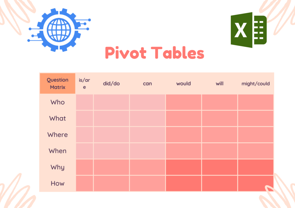
Creating pivot tables in Excel involves several steps. Here’s a step-by-step guide to help you create pivot tables:

Step 1: Prepare Your Data

  • Ensure that your data is well-organized in a tabular format with a clear header row and consistent column names.
  • Remove any empty rows or columns and clean up any unnecessary formatting.

Step 2: Select Your Data Range

  • Highlight the entire data range you want to use for your pivot table, including column headers and all relevant data.

Step 3: Insert a Pivot Table

  • Go to the “Insert” tab in the Excel ribbon.
  • Click on the “PivotTable” button. A dialog box will appear.

Step 4: Choose Your Pivot Table Source

  • Ensure that the “Select a table or range” option is selected in the dialog box.
  • Verify that the correct data range is automatically detected.
  • If necessary, manually adjust the range to include your desired data.

Step 5: Select the Destination for Your Pivot Table

  • Choose whether you want to place your pivot table in a new worksheet or an existing worksheet.
  • If you select an existing worksheet, specify the cell where you want the top-left corner of the pivot table to be placed.

Step 6: Design Your Pivot Table

  • The “PivotTable Field List” pane will appear on the right side of the Excel window.
  • Drag and drop the fields from your data into the appropriate areas of the field list: “Report Filter,” “Column Labels,” “Row Labels,” and “Values.”
  • The “Values” area allows you to specify the summarization of the data (e.g., sum, count, average).

Step 7: Customize Your Pivot Table

  • Use the options in the “PivotTable Field List” pane to further customize your pivot table.
  • For example, you can rearrange fields, change field names, apply number formatting, and apply filtering to focus on specific data.

Step 8: Apply Formatting and Styling

  • Format your pivot table to make it more visually appealing and easier to read.
  • Customize the font, colors, borders, and other formatting options to suit your preferences.
  • Apply any conditional formatting rules to highlight important data or trends.

Step 9: Refresh Your Pivot Table

  • If your underlying data changes or you want to update your pivot table, right-click on the pivot table and select “Refresh” from the context menu.
  • This will update the pivot table with the latest data from your source range.

Step 10: Analyze and Interact with Your Pivot Table

  • Explore and analyze your data using the pivot table.
  • Expand or collapse rows and columns to focus on specific levels of detail.
  • Utilize filtering, sorting, and grouping options to further analyze and drill down into your data.
  • By following these steps, you can create pivot tables in Excel to summarize and analyze your data in a flexible and interactive manner.

Data Symphony: Crafting an Engaging and Insightful Excel Dashboard

Data Symphony: Crafting an Engaging and Insightful Excel Dashboard

Creating an attractive dashboard in Excel involves several steps. Here’s a comprehensive guide to help you create an appealing and functional dashboard


Step 1: Define the Purpose and Audience


  • Determine the purpose of your dashboard. What insights or information do you want to convey?
  • Identify your target audience. Consider their needs, preferences, and level of familiarity with Excel.


Step 2: Plan Your Dashboard


  • Sketch a rough layout of your dashboard on a piece of paper or using a design tool.
  • Identify the key metrics and data that need to be included.
  • Decide on the visual elements, such as charts, graphs, tables, or infographics, that will best represent the data.


Step 3: Gather and Organize Data


  • Collect the necessary data from your data sources, such as Excel spreadsheets, databases, or external sources.
  • Clean and format the data as needed. Remove any duplicates, errors, or irrelevant information.
  • Organize the data into tables or ranges, making it easier to work with later.


Step 4: Choose the Right Charts and Graphs


  • Select appropriate chart types based on the data you want to present. For example, use a line chart for trends, a pie chart for proportions, or a bar chart for comparisons.
  • Ensure that the chosen charts effectively communicate the information you want to convey.


Step 5: Design the Layout


  • Create a new worksheet for your dashboard.
  • Set up a grid system using cells or tables to align your visual elements.
  • Allocate space for titles, headers, legends, and labels to provide clarity and context.


Step 6: Insert Visual Elements


  • Insert charts, graphs, or other visual elements into your dashboard worksheet.
  • Customize each element to match your desired style and design.
  • Resize and reposition elements as necessary to fit the layout.

Step 7: Apply Conditional Formatting


  • Use conditional formatting to highlight important data points or trends.
  • Apply color scales, data bars, or icon sets to make the dashboard visually appealing and easier to interpret.
  • Ensure that the formatting choices enhance the readability and clarity of the data.


Step 8: Add Interactivity (Optional)


  • Create interactive elements, such as drop-down lists, checkboxes, or slicers, to allow users to filter or drill down into the data.
  • Use formulas, such as VLOOKUP or INDEX-MATCH, to make the dashboard dynamic and responsive to user selections.


Step 9: Incorporate Images and Icons


  • Insert relevant images or icons to enhance the visual appeal and convey additional information.
  • Use images sparingly and ensure they are appropriately sized and positioned.


Step 10: Format and Style


  • Apply consistent formatting and styling throughout the dashboard.
  • Use colors, fonts, and font sizes that are visually appealing and easy to read.
  • Align and format text, numbers, and labels for clarity.


Step 11: Test and Review


  • Review the dashboard for accuracy, completeness, and clarity.
  • Ensure that the data is up-to-date and reflects the desired metrics.
  • Test the interactivity, if applicable, to ensure it functions as intended.


Step 12: Protect and Share


  • Protect the dashboard worksheet to prevent accidental changes to the design or data.
  • Save the dashboard as a separate file or a template for future use.
  • Share the dashboard with your intended audience, either by printing it or distributing it electronically.
  • By following these steps, you can create an attractive and informative Excel dashboard to effectively present your data and insights.

Our Partners You trust

Get 1st Exam For Free

Find Your Job Here!

Get A Free Consultation And Estimate